The goal of this assignment is to get our hands dirty in different aspects of image warping with a “cool” application -- image mosaicing. We will take two or more photographs and create an image mosaic by registering, projective warping, resampling, and compositing them. Along the way, we will learn how to compute homographies, and how to use them to warp images.

Shoot the Pictures

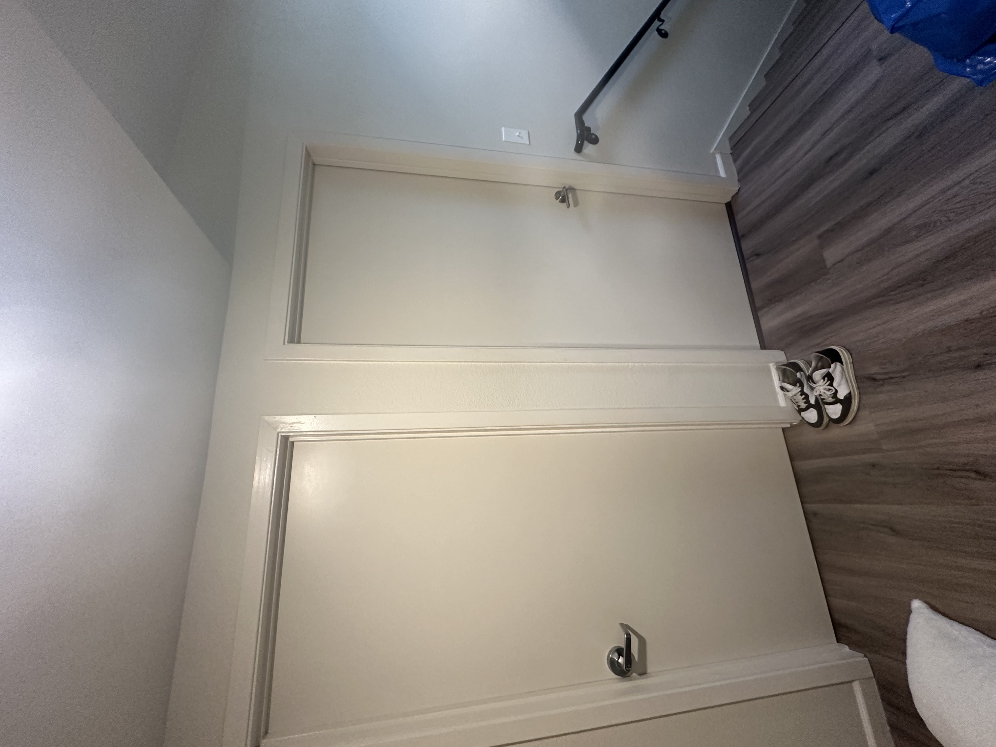
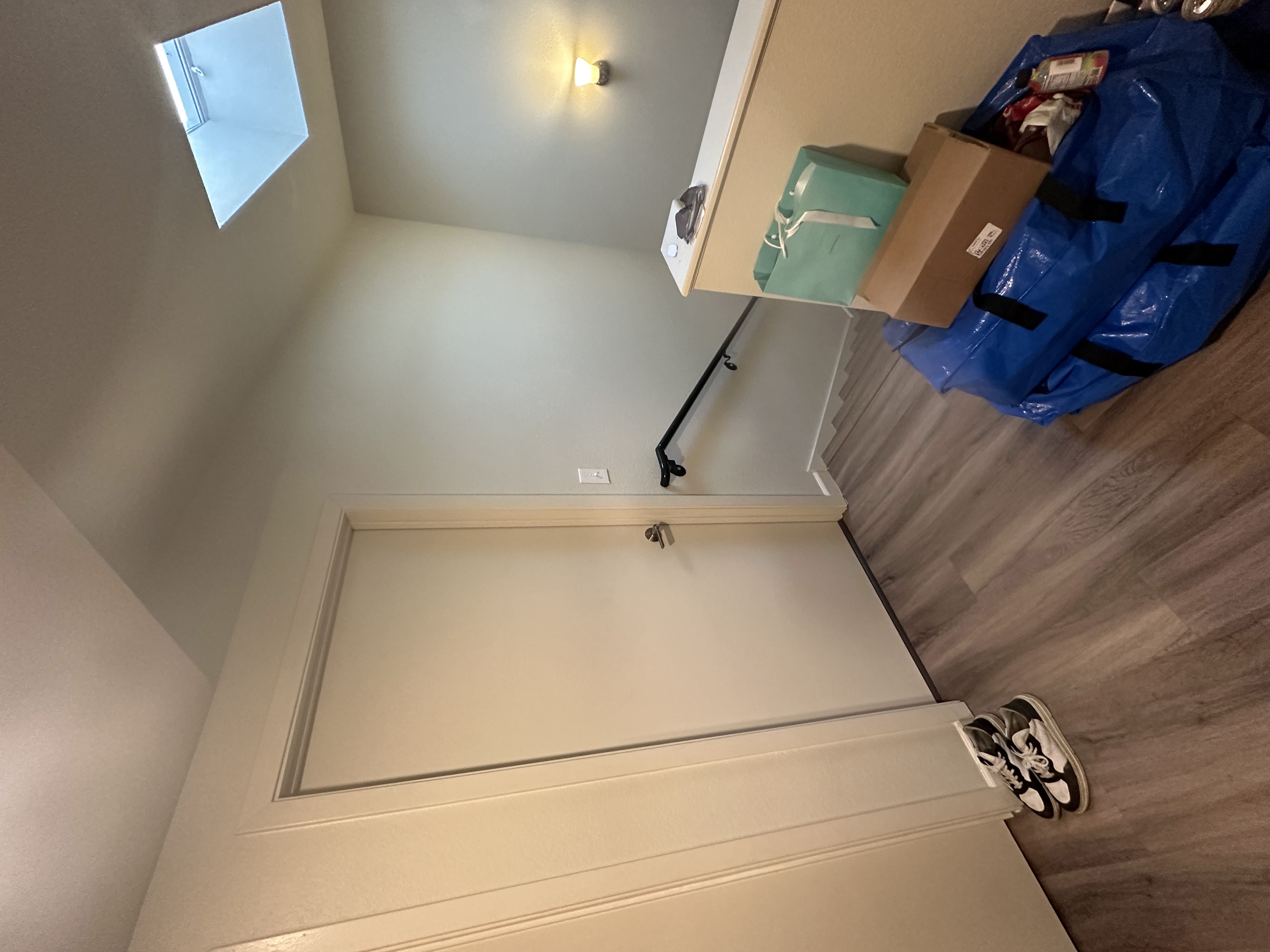
I took a couple of picture sets (2 or 3 imagees) for a few indoor and outdoor scenes that follow the below "rules":

• Projective Transformation: The images should appear to be taken from a single viewpoint, but with a slight rotation or shift between them. This is the essence of projective transformation, where the perspective changes slightly but objects in the scene remain recognizable.
• Sufficient Overlap: Each photo should overlap with the adjacent ones by 40% to 70%. This is crucial for stitching the images together later, as you’ll need common points or features in both images to compute the homography.
• Minimal Distortion: If the images don’t have significant lens distortion (like fisheye or extreme barrel distortion), then they should be fine for your project. If there is distortion, it can complicate the image warping and blending process.
• Consistent Lighting and Scene Stability: If the photos were taken at the same time or under similar lighting, and there’s no significant movement in the scene (e.g., trees swaying too much, water flowing rapidly), then they will work well for image mosaicing.

Recover Homographies

Matrix A Construction

For each correspondence (x₁, y₁) ↔ (x₂, y₂), two rows are added to the matrix A, forming the system:

    [
        -x1, -y1, -1,  0,  0,  0,  x1x2, y1x2, x2
         0,  0,  0, -x1, -y1, -1,  x1y2, y1y2, y2
    ]
    

Solving the System

We use Singular Value Decomposition (SVD) to solve the homogeneous system Ah = 0. The solution vector h (which gives us the homography matrix H) is found from the last row of V^T.

Normalizing the Homography Matrix

After computing the homography matrix H, it is normalized by dividing by the bottom-right value H[2,2] to ensure that the scaling factor is 1.

Warp the Images

Corner Transformation

The corners of the input image are transformed using the homography matrix H to predict the bounding box of the warped image.

Meshgrid for Output Coordinates

We create a grid of output coordinates that span the predicted bounding box. These are the coordinates where we want to compute pixel values for the warped image.

Inverse Warp

We apply the inverse homography H^-1 to map each pixel in the output image back to a coordinate in the input image.

Interpolation

We use scipy.interpolate.griddata to interpolate pixel values at the computed coordinates. This avoids aliasing by smoothly sampling the input image.

Alpha Mask

Pixels that are outside the valid bounds of the input image are marked using an alpha mask or set to zero.

Image Rectification

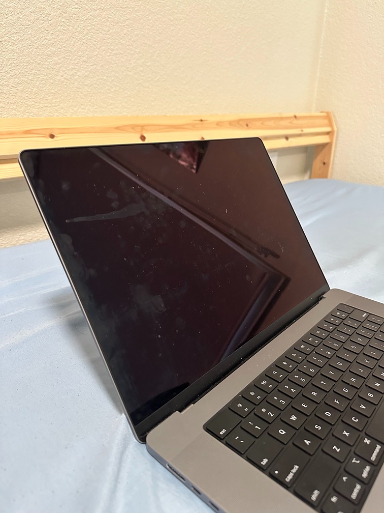
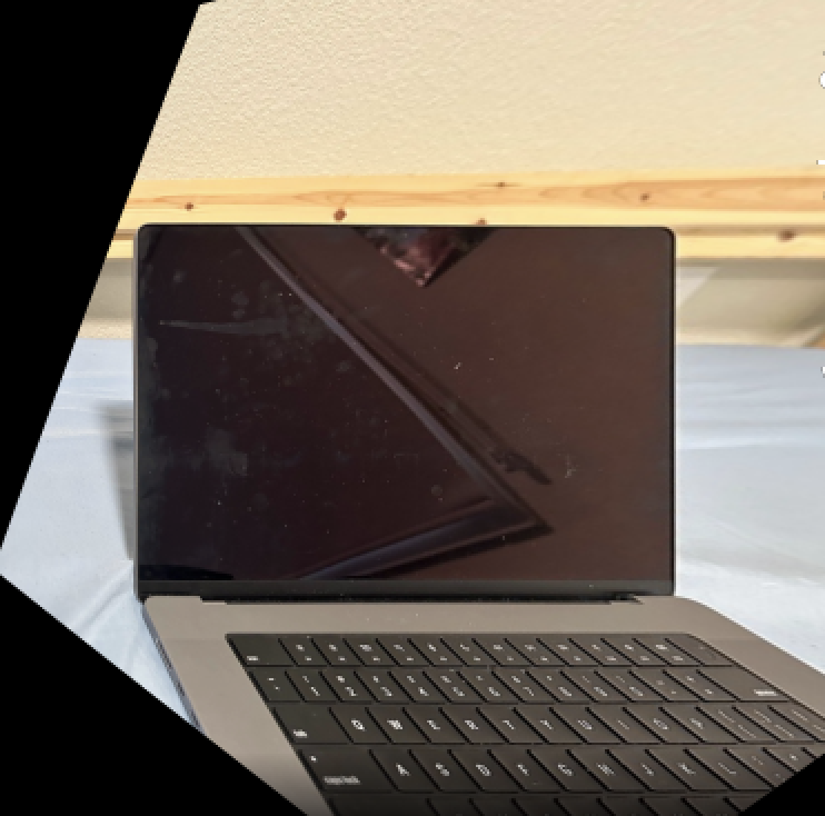
For the process of image rectification, I took a couple of images of rectangular objects, such as a laptop and TV. After which I took the following steps:

Steps for Image Rectification

Define Point Correspondences

• You need to identify four points in your input image (e.g., the corners of a rectangular object like a painting or monitor).
• These points will be stored in im1_pts, representing their coordinates in the image.
• For im2_pts, you define the desired position of these points, typically corresponding to the four corners of a perfect rectangle (e.g., [0, 0], [1, 0], [1, 1], [0, 1]).

Compute Homography

• Using the computeH function that you already developed, compute the homography matrix that maps the points in im1_pts to im2_pts.

Warp the Image

• Use the warpImage function to apply the computed homography and warp the input image so that the rectangular object is rectified.

Visualize the Result

• Display the original and rectified images to verify that the transformation worked as expected.

Below are the results of image rectification

Result-1

Result-2

Blend the images into a mosaic

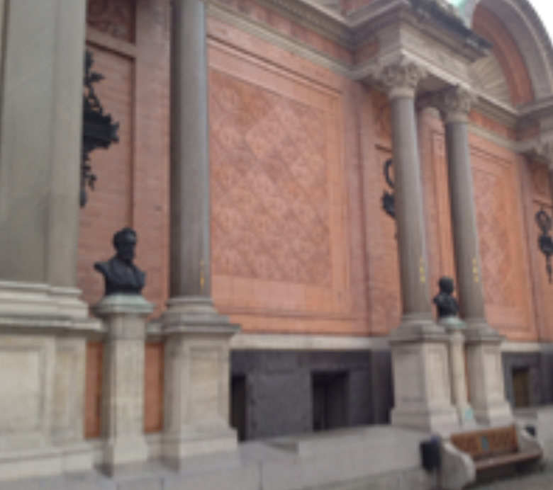
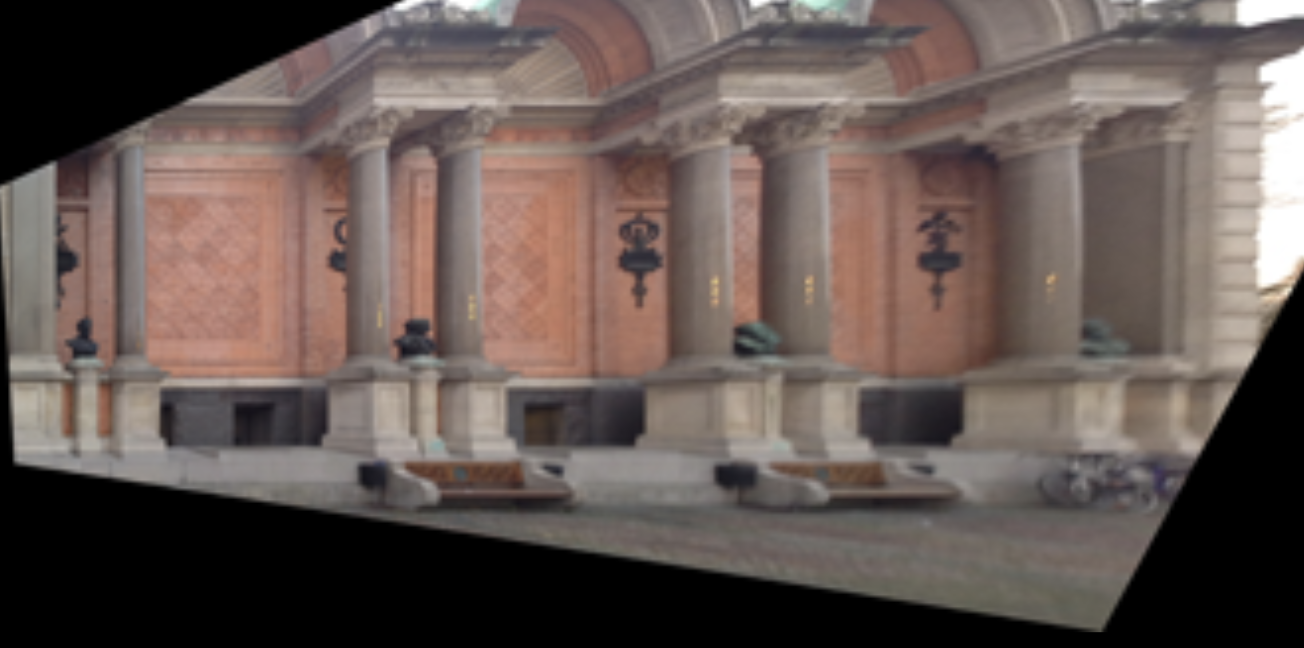
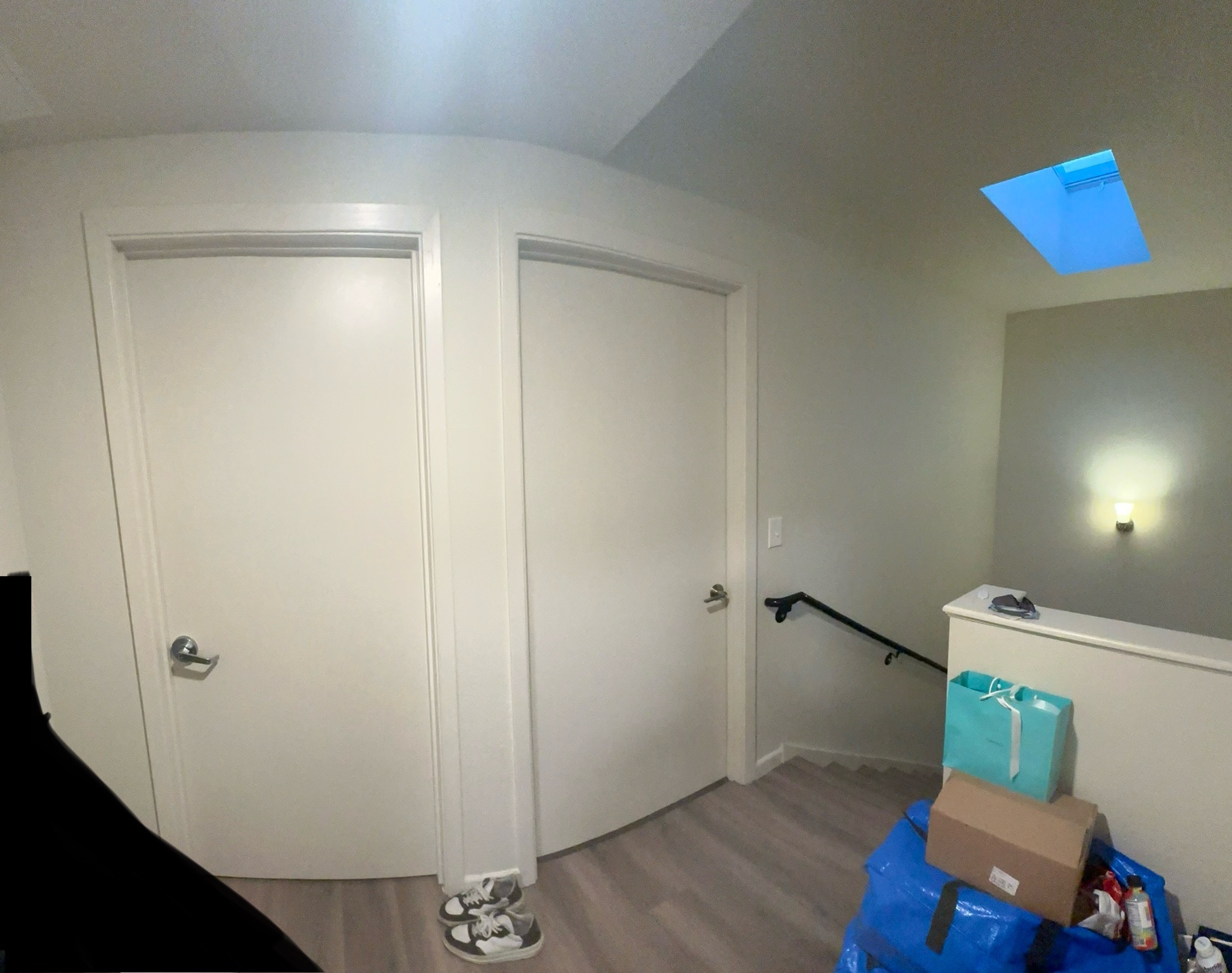
The approach to create a seamless mosaic between two images involves the following steps:

1. Identify Corresponding Points: Manually select common points in both images, such as corners or edges of objects, which will be used to align the images.
2. Calculate Homography Matrix: Using the corresponding points, a homography matrix is computed to map points from the left image to the right (root) image, transforming the perspective.
3. Warp the Left Image: The left image is warped based on the homography matrix so that it aligns with the root image, making their perspectives match.
4. Blend the Images: A blending technique (alpha blending) is applied in the overlapping regions of the two images to ensure a smooth transition without visible seams.
5. Construct the Mosaic: The non-overlapping regions from the left image are combined with the rest of the root image, and the result is a seamless mosaic that includes both images.

Key Concepts

• Homography: Transforms the perspective of one image to match another.
• Warping: Adjusts the left image to align with the root image.
• Blending: Ensures smooth transitions between overlapping parts of the images.

This method results in a combined mosaic that naturally transitions from one image to the other, with aligned perspectives and blended overlapping areas.

Below are the results

Hall Results

TV Results

Kitchen Results

CS 180 Project 4b: FEATURE MATCHING for AUTOSTITCHING

The goal of this project is to create a system for automatically stitching images into a mosaic. A secondary goal is to learn how to read and implement a research paper.

Step 1: Harris Interest Point Detection

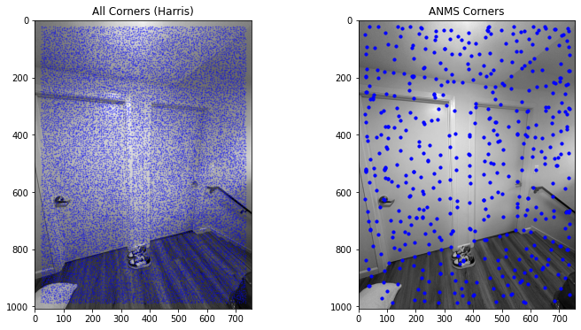
To start, I implemented the Harris corner detector to identify interest points in a single-scale image, following Section 2 of the paper. Rather than developing a multi-scale approach or focusing on sub-pixel accuracy, I simplified the process by using a standard implementation of the Harris detector, provided in harris.py. This function calculates the Harris corner response across the image, highlighting areas with strong corner-like structures.

Once the Harris corners were detected, I overlaid the corner points on the original image to visually represent where interest points were identified. This visualization helped verify that the corner detection was capturing key structural details in the image, which would later be essential for robust feature matching.

Step 2: Adaptive Non-Maximal Suppression (ANMS)

After detecting Harris corners, I implemented Adaptive Non-Maximal Suppression (ANMS) as described in Section 3 of the paper. ANMS refines the set of detected corners by prioritizing points that are not only strong in response but also well-distributed across the image. This step addresses a common issue in feature detection, where too many interest points cluster in certain regions, potentially leading to less effective matching.

ANMS works by selecting a subset of corners based on a suppression radius that adapts according to corner strength. For each corner, I computed the distance to other stronger corners within the neighborhood and retained only those that had a high suppression radius. This ensured a uniform spatial distribution of points, improving the robustness of feature matching in areas of overlap between images. I visualized the final set of selected corners overlaid on the original image to confirm a balanced distribution.

The harris corners and ANMS results are shown as below:

Step 3: Feature Descriptor Extraction

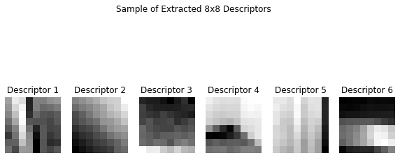
With a refined set of interest points, I proceeded to extract feature descriptors from each selected corner, following Section 4 of the paper. Instead of implementing rotation-invariant descriptors, I simplified the approach by extracting axis-aligned, fixed-size patches, specifically 8x8 patches centered on each corner point. To capture enough context for each descriptor, I extracted each patch from a larger 40x40 window around each interest point.

After sampling, each patch was bias/gain-normalized by subtracting the mean and dividing by the standard deviation. This normalization ensured that the descriptors were invariant to lighting variations, making the features more reliable across images. Each normalized patch was then flattened into a feature vector, which would later be used in the matching step.

Step 4: Feature Matching

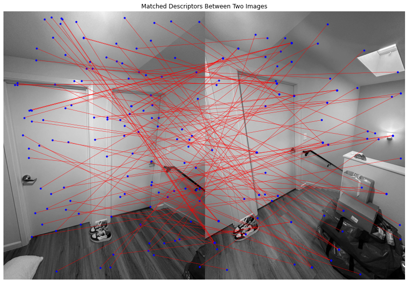
The final step involved matching these feature descriptors between pairs of images. Following Section 5 of the paper and Lowe’s approach, I computed the sum of squared differences (SSD) between each pair of feature descriptors from the two images. For each feature in one image, I identified the nearest and second-nearest neighbors in the other image based on SSD distance. To filter out ambiguous matches, I applied Lowe’s ratio test, which compares the SSD ratio of the closest match to the second-closest match. Only matches with a ratio below a certain threshold were retained, ensuring that each matched pair was unique and distinctive.

This matching process allowed me to identify pairs of points between images that had similar local structures. By visualizing the matches, I could confirm that they were accurate and meaningful, setting up a solid foundation for further steps, such as estimating a robust homography for image stitching.

The Descriptor Extraction and Matching are as below:

Steps to Compute a Robust Homography using 4-point RANSAC

1. Randomly Sample 4 Corresponding Points: Select four pairs of matching points between the two images.
2. Compute the Homography: Use these four pairs to estimate a homography matrix that maps points from one image to the other.
3. Calculate Inliers: Apply the homography to all matching points, then count the number of inliers (points that map closely within a defined threshold).
4. Iterate and Refine: Repeat this process for a specified number of iterations, keeping track of the homography that yields the maximum number of inliers.
5. Return the Best Homography: The homography with the most inliers is the final, robust estimate.

Below are the results

Hall Results

TV Results

Kitchen Results

Takeaways

The coolest thing I learned through this project was the power and versatility of feature-based image matching techniques. Diving into the paper gave me a deeper appreciation for the nuances of computer vision, especially in how robust matching pipelines can be created by carefully balancing detection, descriptor extraction, and spatial distribution of features. The implementation of Adaptive Non-Maximal Suppression (ANMS) was particularly enlightening; I realized how essential it is to ensure a uniform spatial distribution of features to improve matching accuracy and avoid clusters that might introduce ambiguity.

Overall, it was a great learnings experience and a fun project.