CS 180 Project 2: Fun with Filters and Frequencies

This project investigates various techniques for using frequencies to process and combine images in unique ways. Images can be sharpened by filtering and amplifying its higher frequencies. Finite difference kernels can be applied to extract edges. Hybrid images are created by merging the high-frequency components of one image with the low-frequency elements of another. Additionally, images can be blended at different frequency levels using Gaussian and Laplacian pyramids.

Part 1: Fun with Filters

In this part, I built intuitions about 2D convolutions and filtering.

About the gradient magnitude computation

Gradient magnitude computation is a technique used in image processing to measure the strength of changes (gradients) in pixel intensity, typically indicating edges or transitions within an image. It involves calculating the gradient of the image in both horizontal and vertical directions (usually using Sobel or finite difference operators) and then combining these to determine the overall magnitude at each pixel. The gradient magnitude is typically computed as the square root of the sum of the squares of the horizontal and vertical gradients, highlighting regions with significant intensity changes.

Finite Difference Operator

Here are the results of convolving the cameraman image with the finite difference operators Dx and Dy:

1. Original Image: The original cameraman image.
2. Partial Derivative in X: The image after applying the Dx filter, which highlights horizontal edges.
3. Partial Derivative in Y: The image after applying the Dy filter, which highlights vertical edges.
4. Edge Image (Thresholded Gradient Magnitude): The binarized gradient magnitude image, showing the edges. The current threshold value is 0.2.

The edge image can be further refined by adjusting the threshold value to better balance noise suppression and edge detection.

Results

Noticeable Differences

In this task, applying a Gaussian filter before the difference operation serves to smooth the image and reduce noise. When using just the difference operator (e.g., the finite difference), the high-frequency components (such as sharp edges and noise) are amplified, which can result in a noisy output. By first applying a Gaussian filter, we blur the image slightly, which smooths out the noise while preserving important edges.

The key difference is that the Gaussian-smoothed gradient produces cleaner and less noisy results compared to the direct application of the difference operator. Edges appear more defined, while the unwanted noise and high-frequency details are reduced. This results in an overall more visually appealing gradient, with edges more clearly distinguishable. The Gaussian filter effectively suppresses small, abrupt intensity changes due to noise, which helps in producing a clearer representation of the image's true structure.

Image Sharpening

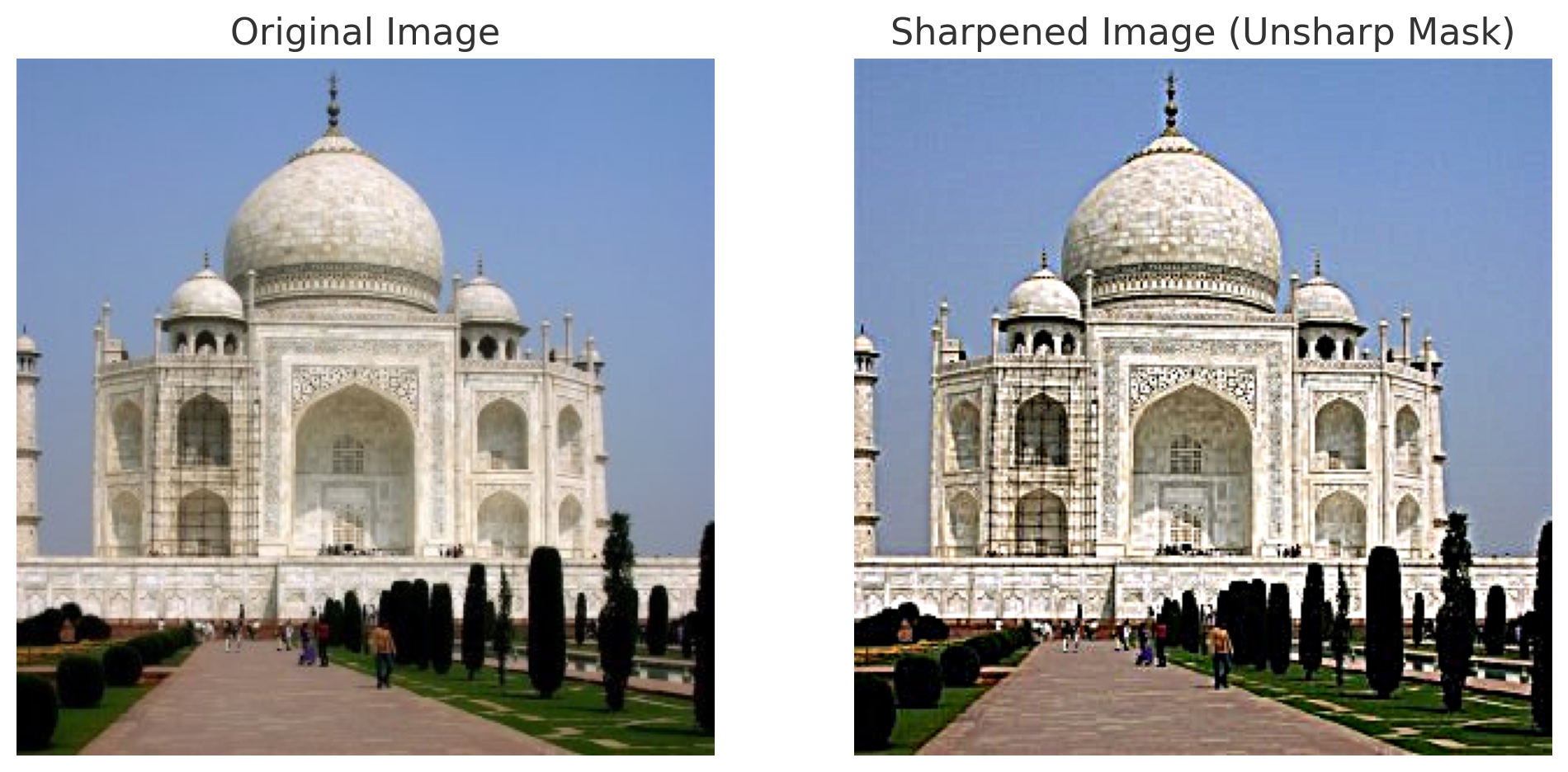
The written code aims to sharpen an image using an unsharp masking technique. The process involves several key steps:

1. Loading and Grayscale Conversion: The image is first loaded, and to simplify the sharpening process, it's converted to grayscale. This reduces the complexity from three channels (RGB) to one (intensity), making the image easier to work with for gradient operations.
2. Gaussian Blurring: A Gaussian blur is applied to the grayscale image. This acts as a low-pass filter, which smooths the image by reducing high-frequency details such as noise and fine texture. The Gaussian filter is created using a 2D convolution, implemented with the cv2.getGaussianKernel() function, generating a 1D Gaussian kernel. The outer product of this kernel with its transpose creates a 2D Gaussian filter.
3. High-Frequency Component Extraction: The blurred version of the image is subtracted from the original grayscale image to isolate the high-frequency components. This captures the details and edges in the image that represent sharp transitions in pixel values.
4. Sharpening: The high-frequency components are added back to the original image (with a scaling factor to control the strength of sharpening). This enhances the details, making the image appear crisper by emphasizing the edges.
5. Display: Finally, the original grayscale image, the blurred (low-pass) image, and the sharpened image are displayed side by side for comparison. This allows for a visual observation of the effect of unsharp masking, where the image is sharpened without amplifying noise excessively, thanks to the Gaussian blur.

This approach ensures that the sharpening process enhances important details while controlling noise, resulting in a visually cleaner output.

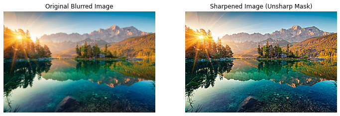
Below, we can see the result after blurring a sharpened image of a waterfall, and resharpening it after. The resharpened image does a good job in recovering most of the lost information.

Hybrid Images

The goal of this part of the assignment is to create hybrid images using the approach described in the SIGGRAPH 2006 paper by Oliva, Torralba, and Schyns. Hybrid images are static images that change in interpretation as a function of the viewing distance. The basic idea is that high frequency tends to dominate perception when it is available, but, at a distance, only the low frequency (smooth) part of the signal can be seen. By blending the high frequency portion of one image with the low-frequency portion of another, you get a hybrid image that leads to different interpretations at different distances.

Results from Running the Code

Gaussian and Laplacian Stacks

Steps for Image Blending

• Gaussian Stacks: The progressively blurred versions of the apple and orange images are displayed.
• Laplacian Stacks: Displayed with contrast enhancement to make the high-frequency details clearer.
• Mask Stack: Shows the progressive blurring of the mask.
• Final Blended Image: Reconstructs and displays the final result of blending the two images.

Multiresolution Blending (a.k.a. the oraple!)

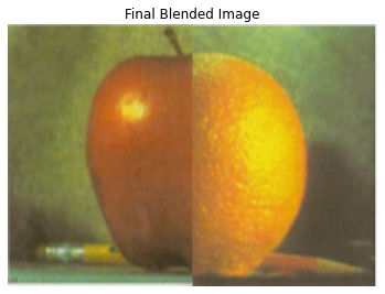
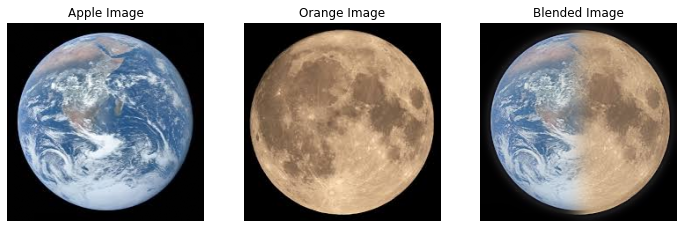
Below is the result of applying the Laplacian Stack to get teh Oraple

Shreyas' Blends Below!!!!

EARTHMOON

WATERMELON DONUT